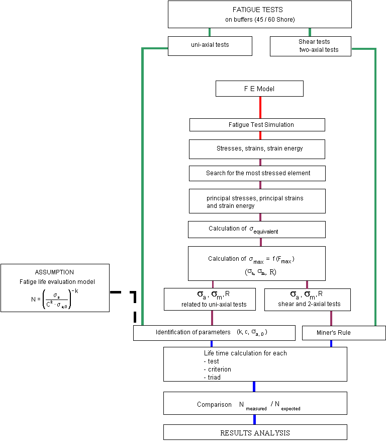
Components made of elastomeric materials own many useful properties, e.g. they endure large displacements, transmit large forces, muffle vibrations etc. Because of the normally non-linear behaviour of elstomers, there exists no common accepted procedure to predict the fatigue life. Therefore, based on experiences received with metallic materials, a special fatigue life model of rubber has been developed and verified by comparison of the life cycles obtained as a result of calculations and experimental tests. A flow chart of the developed procedure is shown in fig. 1
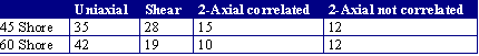
Fatigue tests have been performed varying
- hardness (specimens with 45 and 60 shore) and
- load (uniaxial, shear, 2-axial correlated, 2-Axial non correlated (90 degrees out of phase).
The number of cycles to failure has been defined by the time, when the stiffness shows a defined decline. The total number of experiments performed:
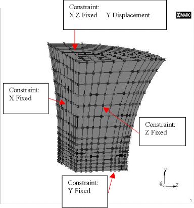
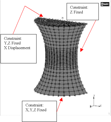
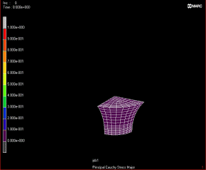
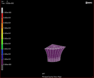
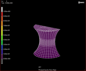
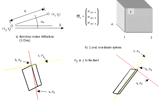
The experimental tests have been simulated by Finite Element Analysis. This is required, because the fatigue life prediction model uses quantities like stresses and strains and usually it is impossible to measure them inside elastomeric components. The mesh used for this application is shown below (fig. 2-3):
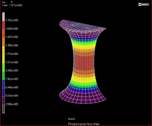
The next step is to determine the maximum stressed element during a load cycle. To perform an exhaustive analysis, principal stresses, strains and strain energy have to be taken into consideration. The appropriate values are determined by analyzing the complete load cycle; this procedure must be performed for all elements because the element with maximum stresses may change in time. The selected elements will be subject of the application of Miner' rule to determine the expected fatigue life. During 2-axial correlated loads simulation numerical problems occured, because the imposed displacements could not be reached and the strain energy showed an high gradient, probably due to a non adequate FE-model. Therefore those results have not been considered. The simulations are shown below (fig. 4 to 7):
The magnitude of the principal stresses and/or strains have to be transformed to an equivalent quantity which can be used to appraise the stresses inside the specimen and to meet the demands of the failure criterion. To reduce the number of computer runs, only that experiment with the largest displacements has been simulated. Therefore the equivalent quantity for the other experiments has been calculated by an interpolation function. This procedure is not adequate for 2-axial non correlated tests, hence in this case all the experiments have been simulated.
The selected forecast model is:
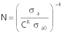
where: {sigma_a, R} define the property of a load cycle and {k, C, sigma_a0} are parameters which characterise the forecast model, calculated by data from uniaxial tests (the reference to analysed complex loads). The model has been used for stresses as well as for strains. The parameters are valid only for a selected material and selected failure criterion. Using strain as the relevant magnitude, the parameters are valid for 45 and 60 shore material at the same time.
Note: the location of principal direction of stress and strain have been calculated to check, wether the load strains always the same fibres; as an example see fig. 8 (uniaxial test). Hence the previous calculations are valid.
The goodness of fit of the forecast model has been evaluated by means of ratios N_measured / N_expected and by visual checks of the Haigh diagrams. The ratios (fig. 9 to 12) show the mean value of a group of tests with same hardness, same failure criterion and same type of load (uniaxial, shear,....). If ratio<1 then life is overestimated, if ratio>1 then life is underestimated.
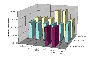
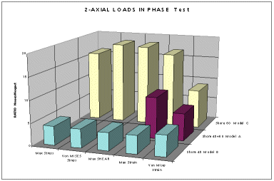
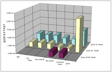
In the previous graphs the quotient N_measured / N_expected do not show relevant differences relative to the failure criterion, therefore all the criteria can be regarded as equivalent. The prediction based on strain energy seems to be not reliable due to obscure interpretations of the F.E.A. results. The results of the "strain-model" (assessment of 45 and 60 shore simultaneously) are close to the others, hence only one relation is sufficient to predict the fatigue life. The difference between load case "2-axial non correlated loads" and the other tests can be attributed to extrapolation problems calculating the equivalent stresses.
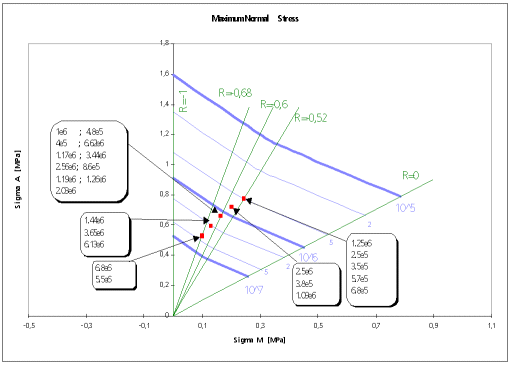
The Haigh diagram is a visual means to evaluated the fatigue life, analyzing all the predicted life cycle values. The results obtained from these diagrams (as example see fig. 13) are the same like above mentioned.
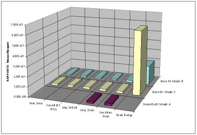
The forecast model provides good results (N_measured / N_expected = 1.5) under simple loads (uniaxial as well as shear). Under "2-axial not correlated loads" N_measured/N_expected = 2.5 and under " 2-axial correlated loads", the ratio arises until about 10.
In all cases fatigue life is underestimated, that means, predictions using this procedure tends to be safe.